
[논문리뷰] Accurate brain age prediction with lightweight deep neural networks (2021)
Updated:
Simple Fully Convolutional Network (SFCN) method 리뷰
논문: Accurate brain age prediction with lightweight deep neural networks, Github
My Preview
regression accuracy를 높일 수 있는 방법으로 교수님이 알려주셔서 리뷰해 본다.
0. Abstract
딥러닝은 질병 예측에 사용할 수 있지만 학습 데이터셋이나 메모리 문제로 성능이 제한적이다. 이런 한계점을 극복하고자 여기서는 Simple Fully Convolutional Network (SFCN)이라는 deep CNN 모델을 제안한다.
SFCN은 기존의 모델들에 비해 파라미터 수가 적어서 양이 적은 데이터셋이나 3D 데이터 학습에 좀 더 적합하다.
성능을 높이기 위해 data augmentation, pre-training, model regularization, model ensemble, prediction bias correction 방법을 함께 사용했다.
1. Introduction
딥러닝 모델은 automatic disease prediction을 위한 도구로 주목받고 있지만 아직 한계점이 있다. 특히 학습 데이터가 3D 데이터인 경우 2D 이미지보다 GPU 메모리를 많이 요구하는 등의 문제점이 있다.
이런 문제를 해결하기 위해 input data를 downsampling 하거나, patch를 사용하거나, 3D 데이터의 2D slice를 사용하거나, reversible architecture를 설계하는 등의 방법들이 연구되었으나 여전히 GPU 메모리 사용량과 information/performance loss 간의 trade-off가 발생한다.
메모리 문제 외에도 medical imaging dataset은 natural image dataset에 비해 sample 수가 적다. 딥러닝 모델 fitting을 위해서는 많은 수의 sample을 필요로 하는데 medical imaging dataset은 데이터의 양이 많지 않아서 image feature를 효과적으로 학습하기 어렵고 overfitting 문제로 이어질 수 있다. 이러한 한계점을 극복하기 위해 새로운 모델 개발이 필요하다.
여기 논문에서는 brain age prediction를 위해 Simple Fully Convolutional Network (SFCN)이라는 가벼운 모델 구조를 제안한다.
SFCN은 fully convolutional network (FCN)과 VGG net을 기반으로 하며 3D T1 brain 영상을 input으로 사용한다.
기존의 VGG net은 (Conv-BatchNorm-Activation)xN-Pooling으로 구성된 basic block을 사용한다. 메모리 효율을 위해 SFCN은 각 MaxPool layer 앞에 conv layer를 하나씩만 둔다. 그리고 모든 fully-connected layer를 제거함으로써 parameter 수를 줄일 뿐만 아니라 input size에 다양성을 준다.
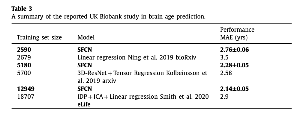
data augmentation과 regularization을 적절히 활용하여 해당 모델은 UK Biobank 데이터셋에서 2.14 (years)의 MAE를 기록했으며, 이는 널리 쓰이는 다른 머신러닝 모델을 사용했을 때보다 좋은 결과이다. 또한 데이터에 여러 가지 방법으로 전처리를 하고 각 결과의 평균을 내는 ensemble 기법을 이용하여 brain age prediction의 accuracy를 더욱 높일 수 있다. 그리고 brain-age delta와 chronological age (실제 연령) 간의 correlation을 크게 줄이기 위해 bias correction 기술을 확장하는 시도도 했다.
2. Methods
2.1. Model: Simple Fully Convolutional Network (SFCN)
Introduction에서 썼듯이 이 모델은 VGGNet 기반이다. 그리고 fully convolutional 구조를 사용하는데, parameter를 3백만 개까지 줄이기 위해 layer 개수를 최소화한다. 이렇게 하면 연산 복잡도와 메모리 사용량을 줄일 수 있다.
SFCN은 일곱 개의 block을 사용한다:
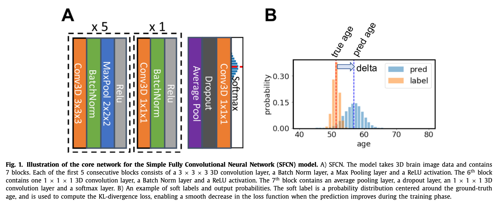
처음 다섯 개의 block은 3x3x3 convolutional layer, batch normalization layer, max pooling layer, ReLU activation layer를 포함한다. 1mm-input-resolution의 160x192x160 3D 영상은 각 block을 feature map을 생성하며 순차적으로 통과하며, 다섯 번째 block 통과 후에 spatial dimension이 5x6x5로 줄어든다.
여섯 번째 block은 1x1x1 convolutional layer, batch normalization layer, ReLU activation layer를 포함한다. 일곱 번째 block은 average pooling layer와 dropout layer(dropout rate은 0.5이고 training 시에만 사용)를 가지며 fully connected layer와 softmax output layer까지 이어진다.
output layer는 40개의 값을 출력하게 되고 이는 1살 간격으로 나눈 42~82세 범위에서 subject가 각 연령에 속할 확률을 예측한 값이다. (The output layer contains 40 digits that represent the predicted probability that the subject’s age falls into a one-year age interval between 42 to 82)
최종 예측값을 만들기 위해 각 age bin의 weighted average를 다음과 같이 계산한다:
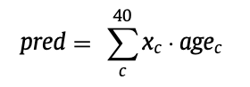
x_c는 c번째 age bin에 속할 확률 예측값이고 age_c는 age 간격의 bin 중심이다.
모델의 process는 3개 단계로 설명할 수 있다.
1) 처음 다섯 개 block이 input image의 feature map을 추출한다.
2) 여섯 번째 block은 nonlinear layer를 하나 추가함으로써 모델의 nonlinearity를 증가시킨다.
이때 feature map의 output size는 안 바뀐다.
3) 일곱 번째 block은 생성된 feature들을 predicted age probability distribution에 mapping 한다.
즉 처음 두 단계는 input image를 feature vector로 인코딩하는 과정이고 세 번째 단계는 deep feature를 이용한 classifier라고 볼 수 있다.
"""코드 출처: https://github.com/ha-ha-ha-han/UKBiobank_deep_pretrain"""
import torch
import torch.nn as nn
import torch.nn.functional as F

class SFCN(nn.Module):
    def __init__(self, channel_number=[32, 64, 128, 256, 256, 64], output_dim=40, dropout=True):
        super(SFCN, self).__init__()
        n_layer = len(channel_number)
        self.feature_extractor = nn.Sequential()
        for i in range(n_layer):
            if i == 0:
                in_channel = 1
            else:
                in_channel = channel_number[i-1]
            out_channel = channel_number[i]
            if i < n_layer-1:
                self.feature_extractor.add_module('conv_%d' % i,
                                                  self.conv_layer(in_channel,
                                                                  out_channel,
                                                                  maxpool=True,
                                                                  kernel_size=3,
                                                                  padding=1))
            else:
                self.feature_extractor.add_module('conv_%d' % i,
                                                  self.conv_layer(in_channel,
                                                                  out_channel,
                                                                  maxpool=False,
                                                                  kernel_size=1,
                                                                  padding=0))
        self.classifier = nn.Sequential()
        avg_shape = [5, 6, 5]
        self.classifier.add_module('average_pool', nn.AvgPool3d(avg_shape))
        if dropout is True:
            self.classifier.add_module('dropout', nn.Dropout(0.5))
        i = n_layer
        in_channel = channel_number[-1]
        out_channel = output_dim
        self.classifier.add_module('conv_%d' % i,
                                   nn.Conv3d(in_channel, out_channel, padding=0, kernel_size=1))

    @staticmethod
    def conv_layer(in_channel, out_channel, maxpool=True, kernel_size=3, padding=0, maxpool_stride=2):
        if maxpool is True:
            layer = nn.Sequential(
                nn.Conv3d(in_channel, out_channel, padding=padding, kernel_size=kernel_size),
                nn.BatchNorm3d(out_channel),
                nn.MaxPool3d(2, stride=maxpool_stride),
                nn.ReLU(),
            )
        else:
            layer = nn.Sequential(
                nn.Conv3d(in_channel, out_channel, padding=padding, kernel_size=kernel_size),
                nn.BatchNorm3d(out_channel),
                nn.ReLU()
            )
        return layer

    def forward(self, x):
        out = list()
        x_f = self.feature_extractor(x)
        x = self.classifier(x_f)
        x = F.log_softmax(x, dim=1)
        out.append(x)
        return out
이 뒤에서는 Introduction에서 말한 것처럼 연산 복잡도와 메모리 사용량을 줄이기 위해 layer를 줄였으며 이를 통해 기존에 많이 사용되던 다른 모델(ex. ResNet)들보다 성능이 좋아졌다는 얘기가 나온다.
2.2. Regression models: Elastic Network
SFCN과의 비교를 위해 Elastic Net 같은 단순한 모델을 사용해 보았다.
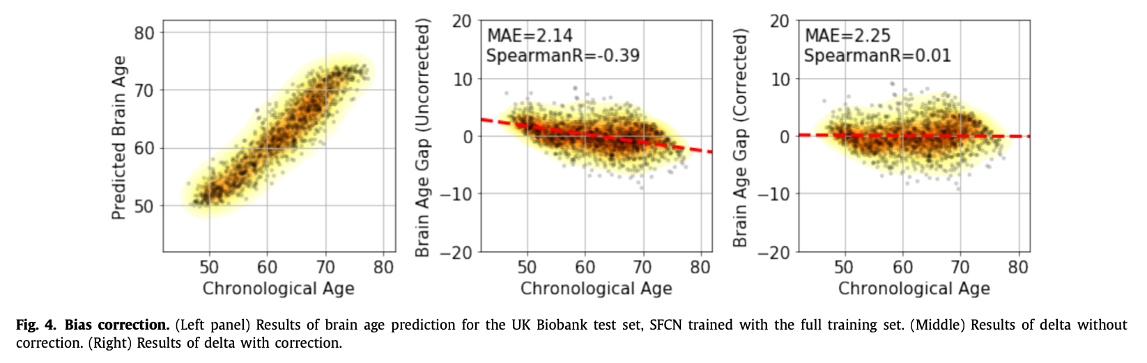
2.3. Bias correction
age delta의 bias에 의한 underfitting 문제를 해결하기 위해 linear bias correction method를 사용했다.
y를 실제 연령, x를 예측한 연령이라고 할 때 validation set에 linear regression x=ay+b를 적용해서 연령 예측값을 x^=(x-b)/a로 correction 하여 계산한다.
3. Experiments
3.1. Datasets and preprocessing
3.1.1 UK Biobank
14,503 subject를 포함하고 있는 UK Biobank 데이터를 사용했다. 여기서 12,949는 training, 518은 validation, 1,036은 testing에 사용되었다. (train:validation:test = 90:3:7, train:validation = 96:4의 비율)
3.1.2 PAC 2019
좀 더 객관적인 성능 평가를 위해 Predictive Analytic Challenge (PAC)에 참여했다. 이때는 전체 2,638개 데이터에서 2,199는 training, 439는 validation에 사용했으며 추가로 660개의 test set이 제공되었다. (train:validation = 83:17) 평가 기준은 brain age prediction에 대해 낮은 MAE와, brain-age delta와 실제 연령 간 spearman correlation이 0.1을 넘지 않으면서 낮은 MAE를 기록하는 것이었다.
3.2. Training and testing
training 할 때 SGD optimizer를 사용했으며 overfitting를 줄이기 위해 training 과정에서 data augmentation 기법을 사용했다. 성능은 validation 및 test set에 대해서 MAE와 Pearson correlation coefficient (r-value)를 가지고 측정했다. (그 외 hyperparameter에 대한 설명 이어짐)
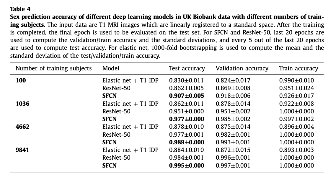
3.3. Sex classification
SFCN의 호환성을 보기 위해 다른 classification 작업도 수행해 보았다.
4. Results
여러 가지 관점에서 결과를 설명하고 있는데 내 관심 대상은 SFCN 모델이므로 모델 성능 평가(4.1)만 자세히 옮기겠다.
4.1. The performance of SFCN in UK Biobank data
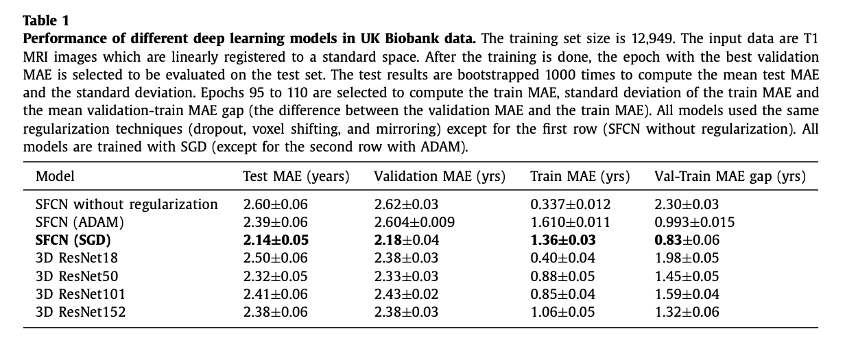
모델 깊이가 깊을수록 성능이 좋아지는 건 아니었다.
hyperparameter tuning 과정에서 optimizer가 모델 성능에 영향을 줄 수 있음을 알았고, 모든 모델 가운데 가장 가벼운 모델인 SFCN이 가장 좋은 성능을 보였다.
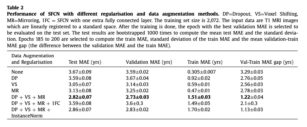
이 연구는 regularization 기술이 모델 성능을 개선할 수 있다는 점과 deep 모델보다 가벼운 모델이 더 나은 결과를 낸다는 점을 보이고 있다.
또한 SFCN은 다른 neuroimaging 연구에도 호환된다. (generalizable)
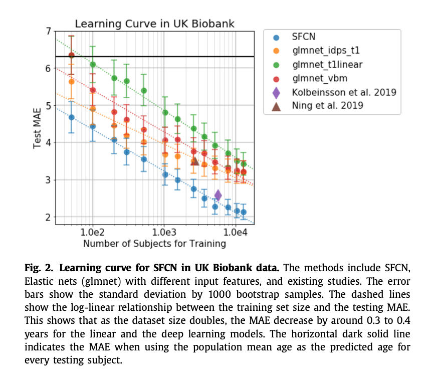
4.2. Comparing the learning curves of SFCN with simpler regression models
4.3. Semi-multimodal model ensemble improves the performance with limited number of training subjects
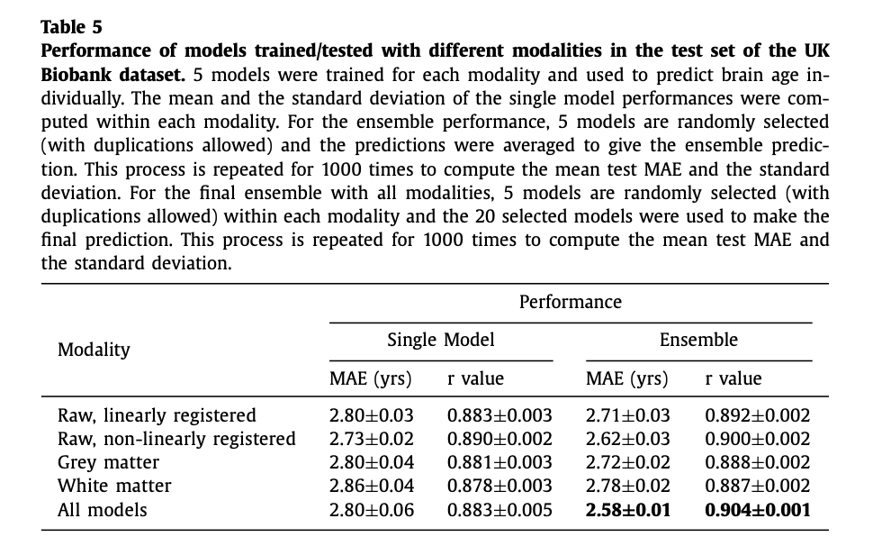
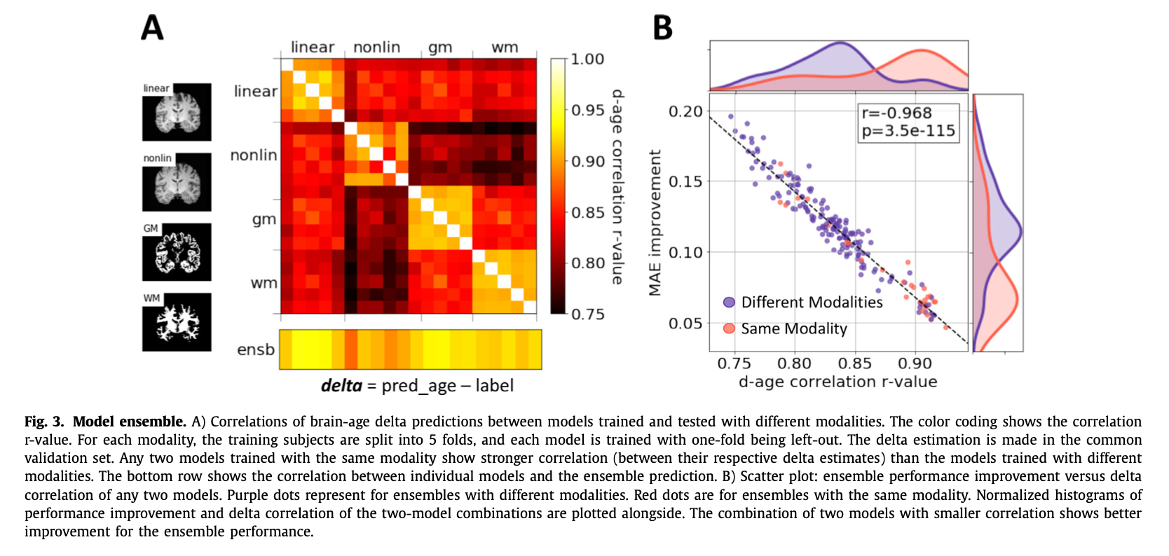
두 개 모델의 correlation이 작을수록 ensemble 성능이 좋아짐을 나타낸다. 다양한 modality에서 학습된 모델들이 correlation이 적기 때문에 서로 다른 modality에 대한 모델을 합치면 성능이 향상된다.
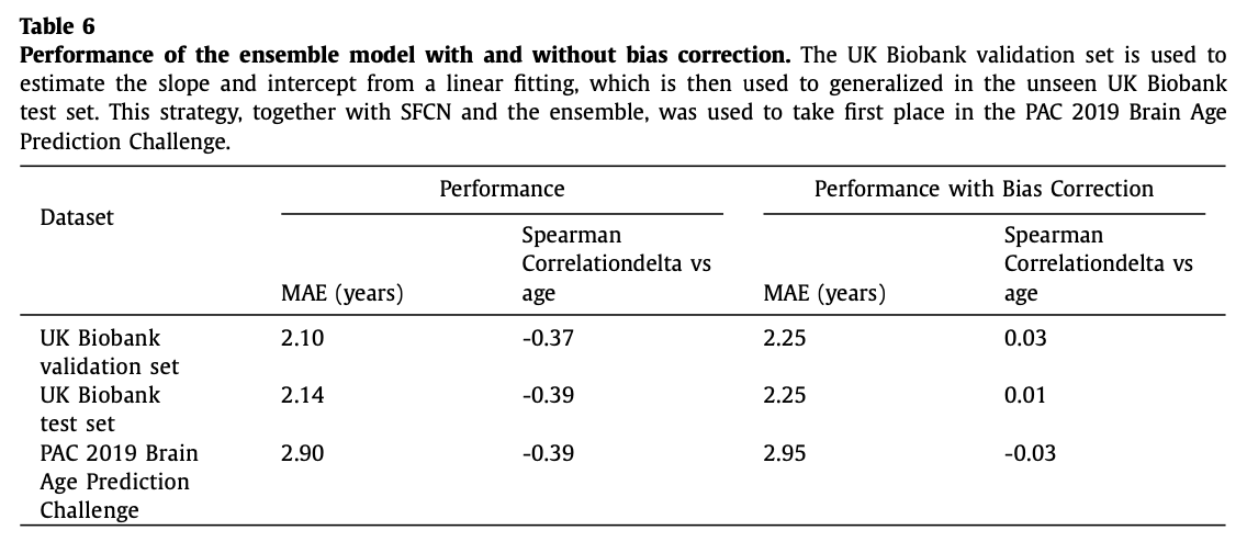
4.4. Bias correction
5. Discussion
이 논문에서는 경량 모델 SFCN의 성능을 입증했다. SFCN은 training set 숫자가 적어도 비교적 좋은 성능을 보이며 기타 neuroimaging data에 대한 deep learning task에도 적용할 수 있다.
Leave a comment