[논문리뷰] RankSim for Deep Imbalanced Regression (2022)

RankSim 논문 & 코드 리뷰

RankSim: Ranking Similarity Regularization for Deep Imbalanced Regression, Github

My Preview

Regularization과 Imbalanced Regression

Regularization이란 weight 값이 너무 커지지 않도록 제한하는 일종의 penalty 조건이다.

한편 regression task가 classification task와 다른 점은 학습 모델이 예측해야 하는 값의 범위가 연속적이라는 것이다. 그래서 imbalanced classification을 위한 method를 regression에 그대로 적용하는 데에는 어려움이 따른다.

전에 정리한 적 있는 Delving into Deep Imbalanced Regression 논문에서는 regression 데이터의 연속성을 이용해서 데이터 분포에 따라 loss를 re-weighting 하거나 (LDS), feature 벡터를 보정하는 (FDS) 방법을 소개하였다. 그리고 오늘 리뷰하고자 하는 이 논문은 거기서 확장해서 regularization을 통해 imbalanced regression의 성능을 높이는 방법을 제안하고 있다.

Introduction

LDS, FDS 등 imbalanced regression 관련 선행 연구와의 차별점: 선행 연구에서는 label space에서 가까이 분포하고 있는 데이터의 관계에 집중하고 있다. RankSim은 label space에서 서로 근처에 있는 데이터 뿐만 아니라 멀리 떨어져 있는 데이터 간의 관계까지 고려하고 있다.

즉 RankSim의 목적은 label space에서 비슷하면 feature space에서도 비슷하라는 것이다.

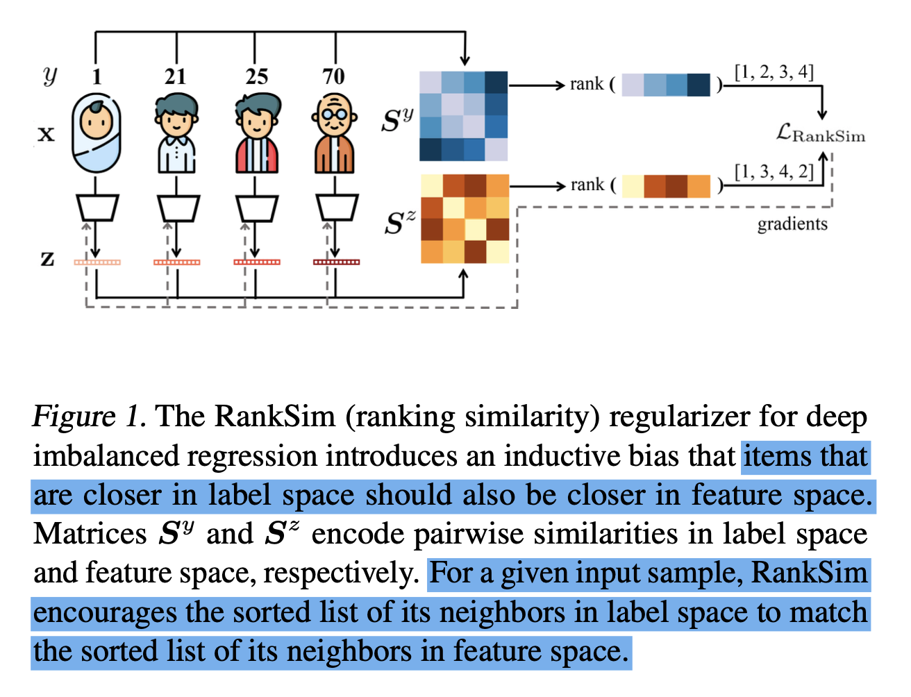
age estimation example에서 1, 21, 25, 70살 데이터를 예로 들어보자.
$ {\bf{z}}^{n} $: label space에서 n살에 해당하는 learned feature
$ \sigma(⋅,⋅) $: 두 벡터 간 similarity function (예: cosine 유사도)
라고 할 때, 21살의 feature인 $ {\bf{z}}^{21} $에 대해서는 $ \sigma({\bf{z}}^{21}, {\bf{z}}^{25}) > \sigma({\bf{z}}^{21}, {\bf{z}}^{1}) > \sigma({\bf{z}}^{21}, {\bf{z}}^{70}) $를 만족하도록 bias를 줘야 한다.

이걸 그림으로 나타낸 게 Figure 1과 같다.

Methods

이 section에서는 수식을 통해 RankSim의 원리를 좀 더 자세히 설명하고 있다.

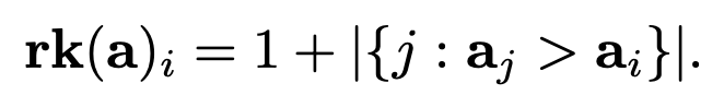
먼저 $ \bf{a}\in\mathbb{R} $ (임의의 실수 n개에 대한 벡터 $ \bf {a} $) 에 대해 ranking function $ \text{rk}(\bf{a}) $를 이렇게 정의한다.

(1)

예를 들어 $ {\bf{a}} = [9,5,11,6] $이면 $ \rm{rk}({\bf{a}}) = [2,4,1,3] $이 된다.

(input, label) 데이터 순서쌍을 $ ({\bf{x}}_i, y_i) $로 표기한다.
$\theta$를 neural network의 학습 parameter라고 하고 $\bf{x}$의 feature를 $ {\bf{z}} = f({\bf{x}};\theta) $로 나타낸다.
RankSim의 아이디어는 $y$와 $\bf{z}$의 순서를 맞추는 데에서 온다.

$ M = \lbrace ({\bf{x}}_{i}, y_i), i=1,…,M \rbrace $ (데이터 순서쌍에 대한 부분 집합)

$ S_{i,j}^{y} = \sigma^{y}(y_i, y_j) $ (2) ($ S^{y}\in{\mathbb{R}}^{M \times M} $, $ \sigma^{y} $: label space에서의 similarity function)

$ S_{i,j}^{z} = \sigma^{z}({\bf{z}}_i, {\bf{z}}_j) = \sigma(f({\bf{x}}_i;\theta), f({\bf{x}}_j;\theta)) $ (3)

(2)와 (3)은 각각 label space와 feature space에서의 $i$ 데이터와 $j$ 데이터의 유사도를 나타낸다.

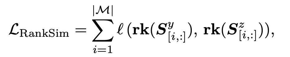
이때 $M$에 대하여 RankSim regularization loss $ L_{\text{RankSim}} $를 다음과 같이 정의한다.

(4)

여기서 $[i,\colon]$은 matrix의 i번째 행을 의미하고 $l$은 input 벡터 간 차이에 페널티를 주는 ranking similarity function이다.

$l$에 mean squared error (MSE)를 사용함으로써 label space의 ranking 벡터와 feature space의 ranking 벡터들 간의 Spearman correlation을 최대화 한다. training 과정에서 각 batch로부터 $M$을 생성하고, 이를 생성할 때는 각 label들이 최대 한 번만 나타나도록 하여 label의 중복을 줄이고 infrequent label과 상대적으로 가까운 값을 좀 더 잘 찾을 수 있게 만든다.

그런데 ranking loss를 다룰 때도 썼지만 ranking 기반 loss는 일부 구간에서 미분이 불가능하기 때문에 모델 최적화에 사용하기 부적절하다. (piecewise constant function라서 거의 모든 구간에서 gradient가 0이 되기 때문.) 그래서 이걸 해결하기 위해 ranking operator를 linear combinatorial objective의 minimizer로 치환한다.

$ {\arg\min}_{\pi\in{\Pi}_n} \bf{a}\cdot{\pi} $ (5)
($ \Pi_n $: ${1,…,n}$의 모든 순열에 대한 집합)

여기서 gradient를 얻기 위해 $\lambda > 0$이라는 interpolation hyperparameter를 사용하여 거의 항상 0이 나올 원래의 gradient 대신에 interpolation의 gradient를 계산한다.

$ \frac{\partial L}{\partial {\bf{a}}} = - \frac{1}{\lambda} (\rm{rk} (\bf{a}) - \rm{rk} ({\bf{a}}_{\lambda})) $ (6)

$ {\bf{a}}_{\lambda} = \bf{a} + \lambda \frac{\partial L}{\partial {\rm{rk}}} $ (7)

이로써 RankSim regularizer를 구현할 수 있고 기존의 training parameter에서 단 두 개의 hyperparameter만이 추가되었다: $\lambda$: interpolation strength, $\gamma$: balancing weight.

Experiments

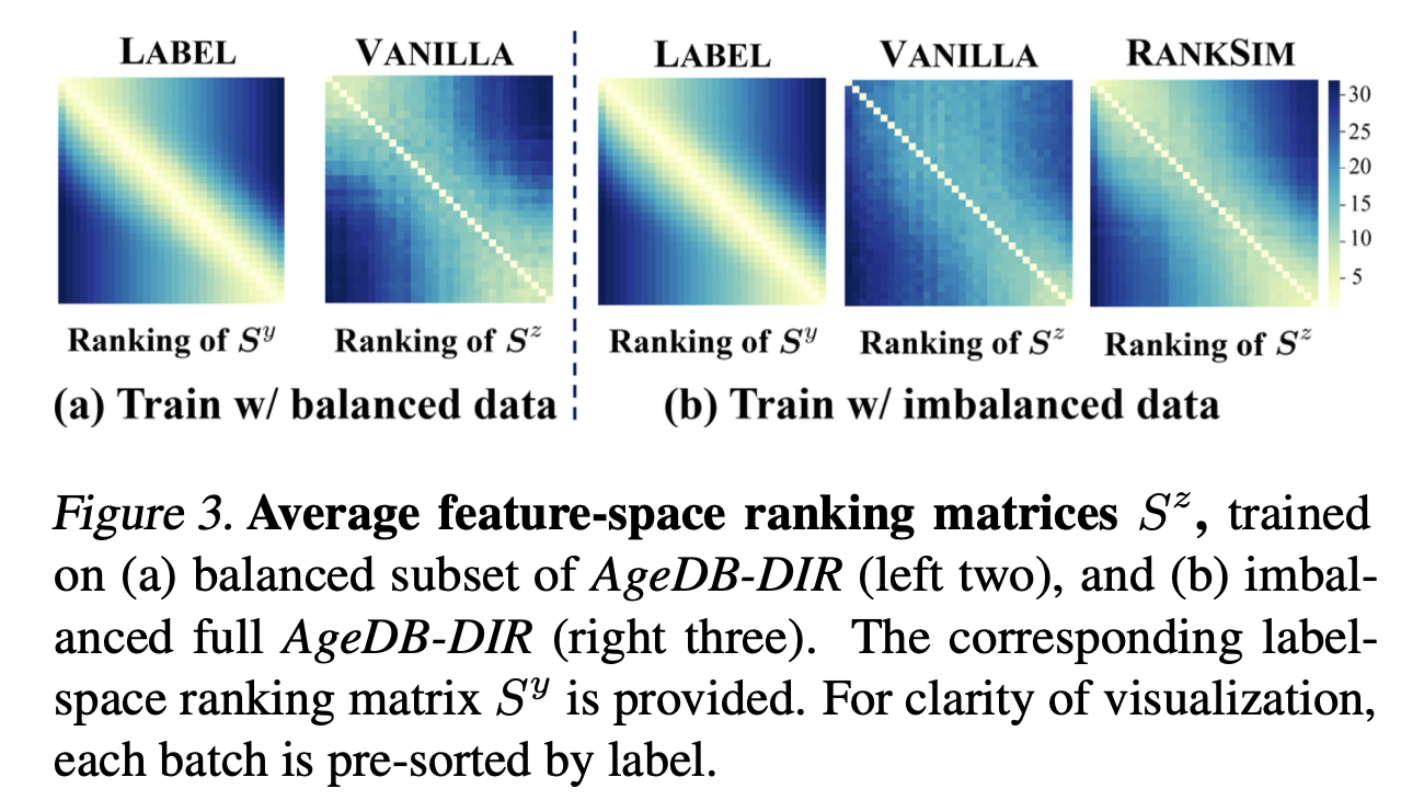
그래서 RankSim을 기존의 imbalanced regression dataset을 가지고 실험해 본 결과 label space에서 인접한 데이터들이 feature space에서도 인접해진 것을 확인할 수 있었다.

Code

어떤 개념인지 알았으니 코드를 살펴보자.

먼저 이 소스코드는 논문에서 제안하고 있는 RankSim regularizer에 해당하는 코드로, 논문에 나와 있는 깃허브 레포에서 가져왔다.

def batchwise_ranking_regularizer(features, targets, interp_strength_lambda):
    loss = 0

    # [1] Reduce ties and boost relative representation of infrequent labels by computing the
    # regularizer over a subset of the batch in which each label appears at most once
    batch_unique_targets = torch.unique(targets)
    if len(batch_unique_targets) < len(targets):
        sampled_indices = []
        for target in batch_unique_targets:
            sampled_indices.append(random.choice((targets == target).nonzero()[:,0]).item())
        x = features[sampled_indices]
        y = targets[sampled_indices]
    else:
        x = features
        y = targets

    # [2] Compute feature similarities for ranking
    xxt = torch.matmul(F.normalize(x.view(x.size(0),-1)), F.normalize(x.view(x.size(0),-1)).permute(1,0))

    # [3] Compute the loss of ranking similarity
    for i in range(len(y)):

        label_ranks = rank_normalised(-torch.abs(y[i] - y).transpose(0,1))
        feature_ranks = TrueRanker.apply(xxt[i].unsqueeze(dim=0), interp_strength_lambda) # differentiable ranking operation, defined in ranking.py
        loss += F.mse_loss(feature_ranks, label_ranks)

    return loss

[1]에서 feature와 target(label) 쌍을 가져오고, [2]에서 feature들 간의 ranking similarity를 계산한다. 그러고 나서 [3]에서 [2]를 이용하여 ranking similarity loss를 구한다 (본문의 (4)번 수식).

[3]의 코드를 보면 rank_normalised랑 TrueRanker라는 처음 보는 메서드가 나오는데 이것도 깃허브에 코드가 올라와 있다. (ranking.py)

# Copyright (c) 2021-present, Royal Bank of Canada.
# All rights reserved.
#
# This source code is licensed under the license found in the
# LICENSE file in the root directory of this source tree.
#######################################################################################################################
# Code is based on the Blackbox Combinatorial Solvers (https://github.com/martius-lab/blackbox-backprop) implementation
# from https://github.com/martius-lab/blackbox-backprop by Marin Vlastelica et al.
#######################################################################################################################
import torch


def rank(seq):
    return torch.argsort(torch.argsort(seq).flip(1))


def rank_normalised(seq):
    return (rank(seq) + 1).float() / seq.size()[1]


class TrueRanker(torch.autograd.Function):
    @staticmethod
    def forward(ctx, sequence, lambda_val):
        rank = rank_normalised(sequence)
        ctx.lambda_val = lambda_val
        ctx.save_for_backward(sequence, rank)
        return rank

    @staticmethod
    def backward(ctx, grad_output):
        sequence, rank = ctx.saved_tensors
        assert grad_output.shape == rank.shape
        sequence_prime = sequence + ctx.lambda_val * grad_output
        rank_prime = rank_normalised(sequence_prime)
        gradient = -(rank - rank_prime) / (ctx.lambda_val + 1e-8)
        return gradient, None

rank_normalised는 본문의 (1)번 수식, TrueRanker는 (6)번 수식을 구현한 것으로 볼 수 있다.

RankSim 구현 방법은 알겠는데 그래서 어떻게 쓰겠다는 거지? training 코드를 보면 어디서 어떻게 쓰는 건지 확인할 수 있다.

for idx, (inputs, targets, weights) in enumerate(train_loader):
        data_time.update(time.time() - end)
        inputs, targets, weights = \
            inputs.cuda(non_blocking=True), targets.cuda(non_blocking=True), weights.cuda(non_blocking=True)

        if args.regularization_weight > 0:
            outputs, features = model(inputs, targets, epoch)
        elif args.fds:
            outputs, _ = model(inputs, targets, epoch)
        else:
            outputs = model(inputs, targets, epoch)

        loss = globals()[f"weighted_{args.loss}_loss"](outputs, targets, weights)

        ## RankSim 사용하는 부분:
        if args.regularization_weight > 0:
            loss += (args.regularization_weight * batchwise_ranking_regularizer(features, targets,
                args.interpolation_lambda))

        assert not (np.isnan(loss.item()) or loss.item() > 1e6), f"Loss explosion: {loss.item()}"

        losses.update(loss.item(), inputs.size(0))

        optimizer.zero_grad()
        loss.backward()
        optimizer.step()

        batch_time.update(time.time() - end)
        end = time.time()
        if idx % args.print_freq == 0:
            progress.display(idx)

cost function으로 batchwise_ranking_regularizer를 사용하고 있음을 알 수 있다. 여기서 regularization_weight과 interpolation_lambda는 본문에서 언급하고 있는 새롭게 추가된 hyperparameter이고, 기본값은 각각 0과 1.0이라고 한다.

regression task 별로 hyperparameter에 어떤 값을 사용했는지도 정리가 되어 있는데,

(1) AGEDB-DIR (age estimation)

$ python train.py --batch_size 64 --lr 2.5e-4 --regularization_weight=100.0 --interpolation_lambda=2.0

(2) IMDB-WIKI-DIR (age estimation)

$ python train.py --batch_size 256 --lr 1e-3 --regularization_weight=100.0 --interpolation_lambda=2.0

(3) STS-B-DIR (natural language dataset)

$ python train.py --regularization_weight=3e-4 --interpolation_lambda=2

이렇게 사용하고 있다.